Predicting Restaurant Revenue with Machine Learning
Our team developed a revenue forecasting model for Restaurant Sonne Sempachersee to address staffing imbalances caused by unpredictable guest volume. By training a Random Forest on four years of sales data, weather metrics, and local event calendars, we built a system that explains 83.22% of revenue variability. This approach reduced forecasting errors by 11.4% compared to the restaurant's existing method, providing a data-driven basis for weekly workforce planning.
This project was developed as part of the Data Science Fundamentals course at the University of St.Gallen (HSG) during the Autumn Semester 2025. I collaborated with my fellow team members Thierry Suhner, Maik Klaiber, and Matthias Hartmann to solve a real-world business challenge for Restaurant Sonne Sempachersee.
The Problem: Guessing How Busy a Restaurant Will Be
Imagine you’re the manager of a lakeside restaurant in Switzerland Restaurant Sonne at Sempachersee. Every Friday evening, you need to decide how many staff members to schedule for the entire upcoming week. You need to know: will Monday be quiet? Will Thursday be slammed? Will the weather bring extra guests to the terrace on Wednesday?
Right now, most small restaurants solve this problem with a simple rule of thumb: look at the same weekday from the past two or three weeks and assume next week will be similar. It’s intuitive, but it’s also pretty inaccurate. The restaurant either ends up paying staff to stand around on a slow Tuesday, or scrambles to serve a full house with half the team on an unexpectedly busy Saturday.
Our project set out to do better by using real historical data, weather information, school holiday calendars, and machine learning models to forecast the restaurant’s daily revenue for an entire week ahead, with enough accuracy to actually improve staffing decisions.
Why This Is a Hard Problem
Revenue forecasting for a restaurant isn’t as straightforward as it might sound. Several factors make it genuinely tricky:
- Weather dependency: A sunny day at a lakeside restaurant means a packed terrace. Rain means half the expected guests might not show up. Temperature, sunshine hours, and rainfall all matter.
- Seasonality on multiple scales: Revenue is higher in summer than in winter, higher on weekends than weekdays, and spikes around school holidays. These patterns nest inside each other.
- Special events: Local events like the Sempacherseelauf (a popular running race), confirmations, and first communions in nearby parishes cause unpredictable revenue spikes. No standard dataset captures these — we had to track them down manually.
- Extreme outliers: Christmas Eve sees almost zero revenue. New Year’s Eve sees the highest revenue of the year by a wide margin. Mother’s Day is also a huge outlier. Any model that tries to “learn” from these gets confused.
Building the Dataset
Good predictions start with good data. We worked with daily revenue records going back to 2021, provided directly by the restaurant owners. On top of that, we assembled several external data sources:
Weather Data
Daily measurements from MeteoSwiss (the Swiss national weather service), specifically from the Luzern weather station:
- Total rainfall (Niederschlag)
- Sunshine duration in hours
- Mean daily temperature at 2 meters above ground
School Holidays
Switzerland’s school holiday calendar is complicated since each canton has different holiday dates. We sourced regional holiday data from official Swiss cantonal holiday calendars to create a continuous indicator of holiday intensity for each day.
Special Days
This was the most labour-intensive part. We manually compiled a list of local events that the restaurant’s business depends on, things like confirmations (Firmung), first communions (Erstkommunion), and the Sempacherseelauf race. For religious events, we called the parish offices directly to get exact dates. There’s no public API for that kind of hyper-local event data.
Birthday Proxy
Here’s a creative one: we used long-term Swiss birth rate statistics (average monthly births over the past 100 years) as a proxy for birthday celebration frequency. More births in a given month → more birthdays → more birthday dinner reservations. It’s an indirect signal, but it adds useful seasonal texture.
Binary Weekend Flag
A simple binary feature marking Fridays and Saturdays as 1, all other days as 0. Despite its simplicity, weekend status is one of the strongest predictors of daily revenue.
Feature Engineering
Raw data alone isn’t enough. We transformed and extended it extensively before feeding it to any model, a process called feature engineering.
Lag Features
We created “lagged” versions of the revenue variable: what was revenue 1 day ago? 7 days ago? 14, 21, 28, 30 days ago? These lag features let the models learn autoregressive patterns, the fact that this Tuesday’s revenue is partly predictable from last Tuesday’s revenue, and the Tuesday before that.
Rolling Statistics
We computed rolling means and standard deviations over windows of 7, 14, and 28 days. This gives the model a sense of recent revenue momentum and variability, is business trending up or down lately? Has it been unusually volatile?
Calendar Features
Month, weekday number, day of year, quarter, and week of year, all extracted from the date. These help models capture the seasonal structure of the data.
Handling Outliers: The Holiday Boost
Rather than trying to model Christmas Eve and New Year’s Eve with a statistical formula (a near-impossible task), we took a pragmatic approach: exclude these extreme days from model training entirely, and replace model predictions on those dates with a manually computed three-year historical average. This is called the Holiday Boost, a post-processing correction that makes the system far more robust around the holiday season.
The Models We Tried
We evaluated five fundamentally different forecasting approaches. All models were evaluated against a naïve benchmark, the simple three-week same-weekday average the restaurant currently uses, which achieved a MAPE of 28.01% and an R² of 0.47.
A quick note on metrics:
- MAE (Mean Absolute Error): Average prediction error in Swiss francs. Lower is better.
- MAPE (Mean Absolute Percentage Error): Average error as a percentage of actual revenue. Lower is better.
- R²: How much of the variance in actual revenue the model explains. Higher is better, with 1.0 being perfect.
Linear & Ridge Regression
This is the simplest approach → fit a straight-line relationship between the features and revenue. We used a Ridge regression with cross-validation to prevent overfitting, with a custom expanding-window time-series cross-validator that simulates realistic week-ahead forecasting. Performance was solid but limited, since revenue has a fundamentally non-linear, seasonal structure that linear models can’t fully capture.
Result: MAE ≈ 2310 CHF | MAPE ≈ 21.83% | R² ≈ 0.77
Random Forest
A random forest is an ensemble of decision trees. It trains hundreds of trees on random subsets of the data and features, then averages their predictions. This makes it robust to noisy, non-linear data and resistant to overfitting in ways that linear models aren’t.
We went through four iterations of progressively more sophisticated setups:
- Baseline Random Forest with 300 trees, max depth 15, minimum 5 samples per leaf
- HistGradientBoosting: a gradient boosting variant that trains trees sequentially, each correcting the errors of the last
- Hyperparameter-tuned Random Forest using our custom
SevenDayForecastCVexpanding-window cross-validation - Fully tuned boosted model with a scaling pipeline, log-transformed target variable (to handle the right-skewed revenue distribution), aggressive hyperparameter search, and bias correction when converting log-predictions back to CHF
The log-transform deserves a brief explanation: daily restaurant revenue is right-skewed, most days earn moderate amounts, but a few exceptional days earn dramatically more. Training on log(revenue) instead of raw revenue stabilizes the variance and reduces the influence of rare spikes, leading to better generalization.
Best Result: MAE = 1953 CHF | MAPE = 16.61% | R² = 0.8322
SARIMAX
SARIMAX stands for Seasonal AutoRegressive Integrated Moving Average with eXogenous regressors, a classical statistical time series model. It explicitly models the autocorrelation structure of the series (how today’s value depends on past values) alongside seasonal patterns, while also incorporating external variables (weather, holidays, etc.) as exogenous regressors.
We enhanced the baseline SARIMAX with Fourier series terms (sine and cosine waves with 16 harmonics) to capture smooth yearly seasonality. Fourier decomposition is a mathematically elegant way to represent complex periodic patterns: rather than forcing the model to learn a rigid seasonal shape, you let it combine sinusoidal waves of different frequencies.
Hyperparameter tuning via grid search over the ARIMA orders (p, d, q) and seasonal orders (P, D, Q) was computationally expensive, and combining it with full cross-validation wasn’t feasible given our resources.
Result: MAE = 2281 CHF | MAPE = 19.01% | R² = 0.77
Prophet
Prophet is a forecasting library developed by Meta’s data science team. It decomposes the time series into interpretable components:
y(t) = Trend(t) + Seasonality(t) + Holidays/Events(t) + Exogenous Regressors(t) + ε
We configured it with an increased changepoint prior scale (0.16 vs. the default 0.05) to allow greater flexibility in detecting structural shifts in revenue. For instance, if the restaurant’s customer base grew significantly in 2023. We also added 16 Fourier terms for custom yearly seasonality and fed in all our engineered features as exogenous regressors.
Cross-validation used an expanding window with a 7-day forecast horizon and an initial training period of 365 days, closely mirroring the real operational use case.
Result: MAE = 2319 CHF | MAPE = 19.83% | R² = 0.7629
LSTM (Long Short-Term Memory Neural Network)
An LSTM is a type of recurrent neural network specifically designed to learn from sequential data. Unlike the models above, it doesn’t require explicit feature engineering to capture temporal patterns, it learns them implicitly through its gated memory cells, which can retain information across many time steps.
Our architecture:
- 30-day sliding window of past daily inputs (revenue + all external features)
- Two LSTM layers with 64 hidden units each
- Fully connected output layer predicting next day’s revenue
- Trained for 50 epochs with the Adam optimizer (learning rate 0.001), batch size 32
We compared a univariate version (only past revenue as input) to a multivariate version (full feature set). The multivariate version improved significantly, as weather, school holidays, and weekend flags provide information that raw revenue history alone can’t capture.
Despite this, the LSTM underperformed relative to the Random Forest. Neural networks generally need large amounts of data to shine, and a few years of daily restaurant records (~1500 data points) is a relatively small dataset for a deep learning approach.
Result (Multivariate): MAE = 2744 CHF | MAPE = 25.65% | R² = 0.6740
Final Results at a Glance
| Model | R² | MAE (CHF) | MAPE (%) |
|---|---|---|---|
| Naïve baseline | 0.47 | 3318 | 28.01 |
| Linear Regression | 0.77 | 2311 | 21.84 |
| Ridge Regression | 0.77 | 2310 | 21.83 |
| SARIMAX | 0.77 | 2281 | 19.01 |
| Prophet | 0.76 | 2319 | 19.83 |
| LSTM (univariate) | 0.62 | 2862 | 26.24 |
| LSTM (multivariate) | 0.67 | 2744 | 25.65 |
| Random Forest | 0.83 | 1953 | 16.61 |
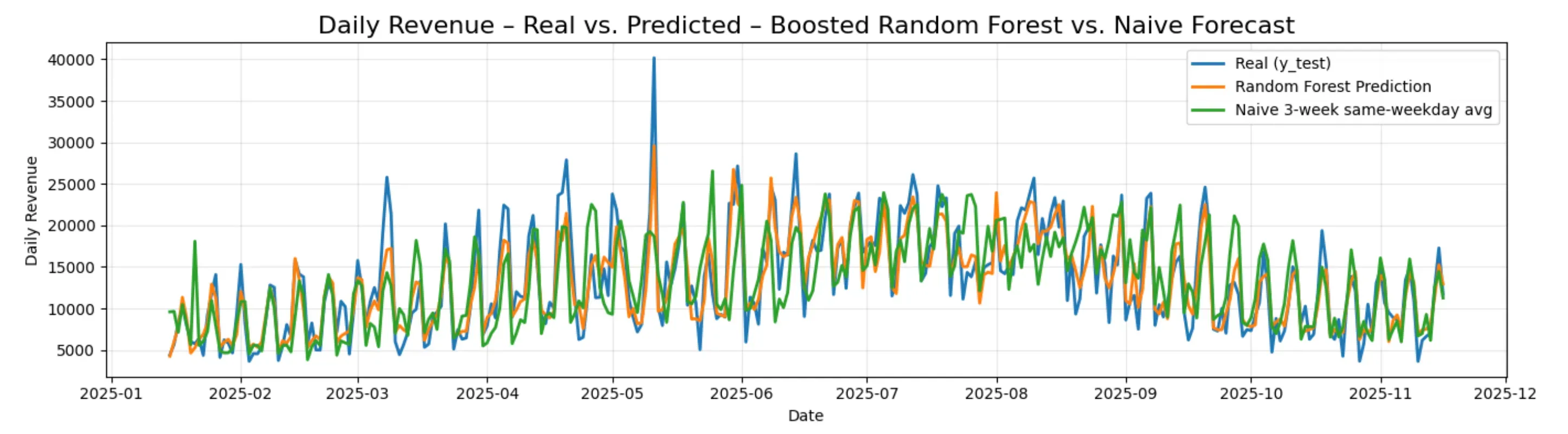
The Random Forest model is the clear winner across all metrics. Compared to the naïve approach the restaurant currently uses, it cuts the average daily prediction error from 3319 CHF to 1953 CHF, a reduction of over 1365 CHF per day. In percentage terms, it improves MAPE from 28% to 16.6%, and its R² of 0.83 means the model explains 83% of the day-to-day variability in revenue.
This project was completed as part of the Data Science Fundamentals course at Universität St. Gallen (HSG), Autumn Semester 2025, Group 8, supervised by Prof. Johannes Binswanger and Prof. Lyudmila Grigoryeva.